StartOut Index Methodology

Methodology for the StartOut Index

The StartOut Index focuses on the impact of high-growth founders from historically underrepresented populations. Research has shown that women, BIPOC, and LGBTQ+ founders, among many others, experience systematic barriers to founding new companies. The Index measures both their existing contributions to their local economies as well as the achievement gaps caused by those barriers.

The initial launch back in 2020 focused on LGBTQ+ and women founders and offered an analysis of interregional inequality. The second iteration launched in October 2022 was about project revitalization and conversion of huge infusion of new data from the 2 additional years into insights for and about LGBTQ+ founders. We updated our industry interactive infographic, as well as implementing front-end changes to enhance the user experience as they navigate through the widget.

For the current iteration of the Index, we are releasing an interactive feature to inform policymakers or anyone looking to get involved on a more grassroots level to discover what policy change or changes could be beneficial or detrimental in terms of funding raised and jobs, patents, or exits created for their local municipality metror state. We used a difference-in-difference model to demonstrate causation between a particular policy, law, ordinance, or regulation funding, jobs, patents, and exits generated by high-growth founders.

For a future release, we plan on incorporating more economic features beyond the US Census Bureau as covariates for our policy data, using different machine learning models to allow for developing insights given recent anti-trans legislation, and developing our race and ethnicity algorithms so that we could start developing metrics around race and ethnicity and gaining some insight into the intersectionality of LGBTQ+ and BIPOC founders.

Funding

As an initial measure of direct economic impact, the Index tracks venture funding and angel investments, as well as other forms of risk capital. The timing, amount, and nature of these investments are derived from the Pitchbook and Crunchbase sources.

The Index applies the same nonparametric estimation algorithm and Metro-based normalization that is used for jobs. This results in the following sub-component

Jobs

“Jobs” is a measure of the number of jobs created by entrepreneurs of our target population in the Metro region within the specified time period. To arrive at this number the StartOut Index records the total number of jobs created by each company located within the Metro. Then, as described above, it credits those jobs to the individual founders of the company. For each founder that is a member of the current target population, the Index adds their share of job creation to its aggregate jobs measure. This provides a total count of jobs created by the target entrepreneurial population.

Because of the issue of undercounting described above, our count of jobs is extended by a non-parametric estimate of the distribution of likely job creation by those undercounted entrepreneurs. To compute this distribution, we sample from the likely number of undercounted entrepreneurs from our target populations. For example, we might have estimated that there’s a 40% probability that 5 of a given Metro’s 200 funded entrepreneurs are likely LGBTQ+ and a 60% probability that 4 of them are LGBTQ+. A distribution over likely job creation is computed as follows:

Randomly select 5 individuals out of the 200.
Count the number of jobs that those 5 individuals created.
Add that number to the set of possible jobs created.
Randomly select 5 new individuals (with replacement) out of the 200.
Count the number of jobs they created.
Add that number to the set of possible jobs created.
Repeat this process until a stable distribution over possible jobs emerges.
Then randomly select 4 individuals out of the 200.
Again, repeat this process using 4 individuals until a new distribution emerges.
Produce a final distribution of likely job creation by weighting the original two distributions by their initial probabilities.

This gives the Index its non-parametric estimated distribution of likely job creation by LGBTQ+ entrepreneurs. If few entrepreneurs in a local population produce jobs then the bulk of this distribution will be 0 additional jobs created. If many entrepreneurs were highly productive, then the distribution accordingly is more likely to include larger job creation values. In either case, it allows us to compute a 99% confidence interval over the likely number of jobs our undercounted population generated. For the sake of Index visualization, this distribution is simplified to its mean, a single value that is added to the job creation sub-factor.

And so the final jobs sub-factor

represents a combination of directly counted job creation and statistical estimate.

The job sub-factor is then normalized to provide a final jobs score

From the aggregate variable

we also compute a mean job score,

The aggregate job score gives the total impact of LGBTQ+ entrepreneurs on job creation within a given Metro. The mean, by comparison, gives us an idea of the individual contributions and challenges of LGBTQ+ entrepreneurs on a one-to-one basis with their straight peers.

Patents

To measure innovation, the Index relies on counts of patents created by each company. (We plan to expand to include research publications and data on media creation in the future.)

Again, the Index applies the nonparametric estimation and Metro-based normalization. This results in the sub-component

Exits

This score measures the total value of all acquisitions and IPOs of companies founded by target population entrepreneurs in a given Metro.

The nonparametric estimation and Metro-based normalization are applied, resulting in the final sub-component

Threshold for High-Growth Company

For the purposes of this Index, we are interested solely in the founders of high-growth companies. As a matter of practical expediency, we laid out a set of minimum criteria to identify high-growth companies in terms of funding or economic impact. To formalize our criteria we began with two company-level data sources focused on the entrepreneurial economy: Crunchbase and Pitchbook.

These sources are the core dataset of the Index. They contain information about companies’ founders, industry, location, funding history, employment and job creation, and exits (e.g. IPOs and acquisitions) and are updated on a regular basis. The Index further augments its dataset with additional information from Wikipedia, the US Patent and Trademark Office, and the US Census Bureau. To credit patent creation to individual founders, the Index traces patent assignment through inventors to employers (companies in our dataset) and finally onto the founders of those companies.

The Index builds this set of high-growth companies and founders based on meeting one of the following criteria:

received any amount of Venture Capital funding, or
received at least $250K in Angel funding, or
generated at least one patent and has created jobs beyond the founding team, or
had an IPO or been acquired by another company.

These criteria allow us to be flexible in our definition of a high-growth company, allowing for organizations that have had an impact even in the absence of institutional funding.

As of the initial launch, these criteria identified 56,623 high-growth companies in the US. As of the second launch, we identified 90,946 high-growth companies in the US.

Founder Identification and Attribution

The purpose of the Index is to measure how individual high-growth entrepreneurs affect metro economies. It constructs this set of individuals using the dataset of high-growth companies described above. An entrepreneur or founder is any member of the founding team, i.e. anyone present at the company before its first round of funding. If a funding date is not available, founders are identified solely from the Crunchbase and Pitchbook labels.

We chose to include people present at a company before first funding, and not just founders, because we believe anyone that joined the company without a promise of funding (or salary) made a formative, high-risk contribution to the company and its impact.

As of our initial launch, our algorithms were able to identify 84,516 high-growth founders. As of our second launch, our algorithms were able to identify 137,661 high-growth founders in the US.

Given a founding team for each company, the Index credits the company’s impact evenly among each of the founders. In other words, for a founding team of 5 individuals, each founder is given credit for ⅕ of the company’s impact (e.g. ⅕ of funding, ⅕ of jobs, ⅕ of patents, and ⅕ of exit value).

Having identified all of the high-growth entrepreneurs in its dataset, the Index applies demographic labels to each: race, gender, and sexuality. To identify LGBTQ+ entrepreneurs, we have integrated three specialized datasets. The first is the membership records of StartOut, the largest LGBTQ+ entrepreneurship group in the world, and Socos’ collaborators in this initiative. The second set of records comes from a data aggregator that provides broad gender and race information to potential employers from 37 publicly available sites. StartOut engaged the aggregator to create a specialized algorithm for identifying LGBTQ individuals in its data. Finally, we have identified a number of public repositories identifying openly LGBTQ+ business leaders, such as Wikipedia.

As of our initial launch, from our database and algorithms, we were able to identify 365 LGBTQ+ high-growth founders, as well as 13,218 high-growth women founders. As of the second launch, from the StartOut database, we were able to identify 774 LGBTQ+ high-growth founders, as well as 17,791 high-growth women founders.

In preliminary work, we found that certain demographic labels such as gender were fairly easily derived from our existing sources. However, as previous research has shown, many LGBTQ+ entrepreneurs are either closeted or at least not public about their identity. This is easy to understand, given that the very same research has revealed the many barriers historically marginalized entrepreneurs have experienced. In addition to the hidden status of many LGBTQ+ entrepreneurs, StartOut’s data overrepresent the cities in which it maintains active chapters: San Francisco, New York, Los Angeles, Boston, Chicago, and Austin. In order to correct for this overrepresentation and known undercounting of LGBTQ entrepreneurs, we have also developed a statistical model to estimate counts over our outcome variables of interest.

The StartOut Index employs a statistical estimate of the undercount of founders. It estimates a distribution over the likely number of hidden LGBTQ+ founders in each Metro. The initial estimate of LGBTQ+ entrepreneurship rate is calculated through a simple linear regression. The linear regression formula is shown below:

where lgbtq_founder_rate is the number of counted LGBTQ+ founders, all_founder_rate is the total number of founders divided by the total population count, and lgbtq_pop_prop is the percentage of known LGBTQ+ population from UCLA’s Williams Institute.

After training this linear regression model with the best in class metros (San Francisco Bay Area and New York), all metros have an estimated LGBTQ+ founder rate. The best in class metros give a starting point in estimating what could be the total proportion of LGBTQ+ founders for each metro.

After this step, each metro will be assigned the estimated number of LGBTQ+ founders. Since this is a rough estimate, the next step is to run some simulations for each metro to get a better estimate of the number of LGBTQ+ founders for each metro. The simulation looks to optimize the estimated number of LGBTQ+ founders, iteratively stepping through estimates. The end result is a better approximation for the number of LGBTQ+ founders for each metro.

To calculate the estimated number of undercounted founders, subtract the estimated number of LGBTQ+ founders from the counted number of LGBTQ+ founders in the dataset. Subsequently, the number of undercounted LGBTQ+ founders will be used to estimate the undercounted funding, jobs, patents, and exits for LGBTQ+ founders, per metro.

All identities of entrepreneurs in the system, LGBTQ+ or otherwise, are anonymized for publication and used for no other purpose than producing the Index.

At the time of launch, these criteria identified 84,516 high-growth entrepreneurs.

At the time of the second launch, we have identified 124,756 high-growth entrepreneurs in the US.

Estimating LGBTQ+ Founder Subfactors

Now that each metro has an assigned estimated number of undercounted LGBTQ+ founders, the next step is to perform further simulations. This next step will result in a distribution of the undercounted LGBTQ+ founders, funding, jobs, patents, and exits for a particular metro. For each metro and for each simulation run, sample from a Poisson distribution with the mean being the estimated number of undercounted LGBTQ+ founders from the previous subsection. With this number, sample that many founders from a particular metro, keeping track of the funding, jobs, patents, and exits associated with each sample. The results from these simulations, for each metro, is a distribution of numbers for the undercounted LGBTQ+ founders, funding, jobs, patents, and exits. An empirical confidence interval can be calculated using quantiles to give a good idea of the range of the estimated values.

The sampling of founders from the previous paragraph is described here. Given an estimated number of founders to sample, each sample will sample from the founders with an unknown LGBTQ+ identity for a given metro. This effectively results in simulating the estimated, undercounted funding, jobs, patents, and exits for a given metro. The sampling procedure is similar to a multinomial distribution, where each founder in a given metro is assigned a probability of being LGBTQ+. However, in this algorithm, the sampling occurs without replacement. Founders with an unknown LGBTQ+ identity are each assigned a number, where a larger number means this founder will be more likely to be sampled.

This number is calculated by, first, calculating industry ratios for each industry in a given metro. For each metro, the count of known LGBTQ+ founders and the count of unidentified LGBTQ+ founders (they either don’t identify as LGBTQ+ or their identity is unknown) are recorded for each industry. One example is the following: there are only two industries in a particular metro: Social Media and Technology. For this particular metro, there are 8 LGBTQ+ founders working in Social Media, 2 LGBTQ+ founders working in Technology, 20 unidentified LGBTQ+ founders working in Social Media, and 80 unidentified LGBTQ+ founders working in Technology. Thus, 0.8 of LGBTQ+ founders are working in Social Media, 0.2 of LGBTQ+ founders are working in Technology, 0.2 of unidentified founders are working in Social Media, and 0.8 of unidentified founders are working in Technology.

Next, for each industry, a ratio of LGBTQ and unidentified LGBTQ+ is calculated. The Social Media ratio is 0.8 / 0.2 = 4 and the Technology ratio is 0.2 / 0.8 = 0.25. Each industry in a given metro has an associated industry ratio. Any founder may be associated with a particular industry in a particular metro; for each industry an founder is associated with, the corresponding industry ratio is added to the founder’s total and then averaged based on the number of industries that the founder is in. To sum, the industry ratio is a measure of how likely it is for LGBTQ founders to be in that industry compared to the unidentified LGBTQ founders. A higher ratio indicates that, for that particular industry in the metro, there is a higher proportion LGBTQ+ founders in that industry than the unidentified. founders with a higher average industry ratio will be more likely to be sampled from this simulation, implying that they are more likely to be LGBTQ because of the associated industries they are in.

Now that the issues with undercounting LGBTQ+ founders have been addressed, the following sections include statistical analyses on founders across these metros. The section titled Index v2.0 highlights the methodology behind the Entrepreneurship Equity Score and the Impact Score. The section titled Policy v1.0 also provides the details of the statistical work behind the policy recommendations.

Metros

The core entity of the Index is the Metro, derived from the census bureau’s definition of metropolitan statistical area. Metros represent large integrated economic regions. For example, the entirety of the San Francisco Bay Area–Oakland, San Jose, Marin County, and more–are all assigned to San Francisco Metro. The impact of individual entrepreneurs and founders on a Metro is measured in terms of the location of the headquarters of companies they have founded. This means that some prolific founders have had impacts across multiple Metros. This also means that impact measures such as jobs and patents are treated more as indices than explicit economic activity as they are credited back to the founding metro region even if the jobs actually exist in a separate city. Lastly, to be considered as qualified, a metro area has met the minimum threshold of 50 qualified entrepreneurs.

At the time of launch, these criteria identified 77 Metros in the United States.

At the time of the second launch, 118 Metros in the United States have been identified as qualified.

Entrepreneurship Equity Score

The Entrepreneurship Equity Score (EES) is a score that represents an estimate of founder success of a specific founder group. This score is a function of funding, jobs, patents, exits, and achievable funding, jobs, patents, and exits. The pre-standardized EES is defined below:

where i represents a particular Metro, j represents an founder group, and k represents a target. The standardization process, which will standardize the scores between 0-100, will be described at the end of this section.

This score is calculated for each unique combination of founder group (All, LGBTQ+, Women) and target (total, mean). Each metro will obtain an EES based on their founder performance given a specific founder group and target. This implies that all of the calculations for EES will be separately computed for each metro, founder group, and target. These calculations include: aggregated target subfactors, best in class metros, and achievable target subfactors. The definitions for these calculations will be discussed later. For example, if the founder group is LGBTQ+ and the target is total, then the EES will be calculated using the aggregated total LGBTQ+ subfactors, the corresponding best in class metros using the total LGBTQ+ subfactors, and the achievable total LGBTQ+ subfactors. If the founder group is LGBTQ+ and the target is mean, then the EES will be calculated using the aggregated mean LGBTQ+ subfactors, the corresponding best in class metros using the mean LGBTQ+ subfactors, and the achievable mean LGBTQ+ subfactors. The scores are similarly calculated for All and Women founders as well.

The achievable subfactors are estimates of potential funding, jobs, patents, and exits that could have been achieved, given equal access to resources. Each metro will have achievable funding, jobs, patents, and exits associated with it. For each subfactor, the achievable is calculated by first finding the best in class comparison ratio across the metros. These comparison ratios are calculated differently, depending on the given founderial group. To manage outlier entrepreneurs in each metro, the top 5 entrepreneurs and their corresponding subfactors were removed from the achievable calculations, for each metro. This mitigates some of the issues with outstanding entrepreneurs that would push the average subfactors to extreme numbers.

For the LGBTQ+ founder group, the comparison ratio for a given subfactor and target is defined as the aggregated target subfactor for LGBTQ+ founders divided by the aggregated target subfactor for non-LGBTQ+ founders (the use of “non” is precarious because there is no certainty in the identification of LGBTQ+ people or non-LGBTQ+ people in the data; this is the case for Women founders as well). For example, for each given metro, if the target is total and the subfactor is funding, the comparison ratio is calculated by taking the total funding raised by LGBTQ+ founders divided by the total funding raised by non-LGBTQ+ founders. This comparison ratio demonstrates how well LGBTQ+ founders are doing in terms of raising total funds compared to their counterparts. A ratio of 1 indicates that LGBTQ+ founders are doing equally as well as their counterparts in terms of total funding. A ratio greater than 1 indicates that LGBTQ+ founders are doing exceptionally well compared to their counterparts in terms of total funding. Thus, each metro has a total funding comparison ratio for LGBTQ+ founders. The top 3 metros with the largest comparison ratios are considered the best in class in terms of total funding for LGBTQ+ founders. Similarly, the best in class metros and their comparison ratios are calculated for the remaining subfactors.

Similarly, for the Women founder group, the comparison ratio for a given subfactor and target is defined as the aggregated target subfactor for Women founders divided by the aggregated target subfactor for non-Women founders.

For the All Founders group, the best in class is defined differently. Instead of a comparison group, the top 3 metros are ranked by the top 3 GDP per capita. For these top 3 metros, their mean subfactors are also recorded.

Now that the best in class metros are determined for each subfactor, target, and enterpreneurial group, the achievables can be calculated.

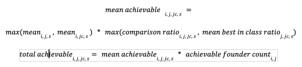
where i represents a particular Metro, j represents an founder group, jc represents the founder comparison group, and s represents a subfactor.

The above formulas define the mean achievables and total achievables for each subfactor for every given metro and founder group with their corresponding founder comparison group. These definitions implicitly account for everything unique about metro foundership rates, access to capital, number of universities, and more – and only adjusting for the relative performance of the target population. The definitions assume that these founder groups can meet the same best in class productivity ratios in their metros.

One important thing to note is that the achievable founder count is calculated by finding the mean best in class founder rate and dividing it by each metro’s founder rate. This proportional ratio is then multiplied by the number of founders in each metro, resulting in the achievable founder count.

Now that the achievables are calculated, the pre-standardized EES from above can be computed. Each metro now has a pre-standardized EES, each with scores for the separate founder groups and targets. Next, each EES will be standardized to a score between 0-100; these scores will be standardized by each unique founder group and target. The standardization process includes forcibly creating a normal distribution out of the scores i.e. a majority of scores will have scores closer to 50 with a few scores at the tail ends. Due to a lack of reported founder data in several metros, these metros were assigned a minimum index score of 1.

Metros with a large EES include a founder group that is doing exceptionally well in terms of economic activity compared to their counterparts. These metros are generally the metros that are considered best in class, given the founder group and target. On the other hand, metros with a small EES have a founder group that is not doing as well compared to their counterparts. Ultimately, these scores highlight thriving and up-and-coming metros with high-growth startups. These scores also stress the necessity to support underrepresented groups, especially LGBTQ+ founders.

Impact Size

The Index produces two main components: the Index Score and the Impact Size. The Score is a measure of the achievement gap for the given Metro region and will be discussed further below. The Impact Size is an absolute measure of the economic impact of our population of interest, i.e. LGBTQ+ entrepreneurs.

The Impact Size is computed by adding the four normalized sub-factors together to give a measure of the “economy” for LGBTQ+ entrepreneurs

Similarly we compute a mean impact size to reflect the average impact of individual LGBTQ+ entrepreneurs in a given metro

Industry Fingerprint

To begin to explore the causes behind the achievement gap, the Index analyses likely factors that set the context for entrepreneurial success. One particularly relevant factor is the relative composition of industries within a given Metro region. The Index computes an industry fingerprint for each Metro to provide a visual summary of inclusion at the industry level.

To create this fingerprint, the Index uses the Global Industry Classification Standard (GICS) to count the number of companies in each industry. (Individual companies were allowed to be counted in more than one industry.) These counts were then normalized by the total number of companies in a given Metro, giving a proportion of industry in the Metro economy. Industry proportions were also computed at a national level. Finally, for each industry in each Metro, a likelihood ratio was computed by dividing the Metro proportion for that industry by the national proportion. This ratio indicates whether a given industry is over- or under-represented in a local economy compared to the nation at large.

For each Metro, the Index computes an industry weight as

where i is each Metro.

The Index computes an industry gap as a weighted average of the individual impact scores by the industry weights

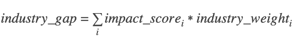
The industry fingerprint then represents the size of the industry across all entrepreneurs within the Metro (target and comparison) as well as the weighted average of the achievement gap across the target population for the entire nation. This offers some insight into why a city might be particularly challenging or successful for a given target population.

Policy v1.0

Non-Policy Data

We collected non-policy data predominantly from the United States Census Bureau consisting of 247 different sociological and demographic features for every state and 186 for every qualifying metro in our selected years of 2010 and 2020. Economic data was collected from the Census Bureau, but supplemented with data from FRED, BLS, and BEA. When data was unavailable for 2010 and 2020, we substituted data from the previous or subsequent years.

Data included age, gender, race, ancestry, place of birth, marital status, household and families, occupancy characteristics, children characteristics, means of transportation, commuting characteristics, educational attainment, school enrollment, nativity and citizenship status, language spoken at home, income and earnings, employment status, occupation, industry, poverty status, veteran status, voting status, as well as other social, economic, housing, financial, and economic characteristics.

We attempted to collect data on every state and territory in the United States, i.e. DC, Puerto Rico, Guam, etc. For the qualifying metros, we matched the metros to existing Combined Statistical Areas (CSA) first and then any remaining metros to Metropolitan or Micropolitan Statistical Areas (MSA/uSA). One notable exception is splitting the Washington DC CSA back into the Washington DC and Baltimore MSA’s since they are very distinct and different founder spaces. There are currently 119 qualifying metros: 63 of the metros were in CSA’s in 2010 while 87 of the metros were in CSA’s in 2020.

We relied on the Williams Institute as our resource for demographic data on the LGBT community on state-level and metro-level including racial makeup by state and metro area, age distribution, and socioeconomic indicators. We use such data to calculate our estimated numbers for LGBTQ+ founders in a given metro or state based on our top 3 best-in-class in the respective geographic region.

Policy Data

Our policy data were collected from the Movement Advancement Project (MAP) and Fraser Institute Economic Freedom Rankings. MAP covers 50 different LGBTQ-related laws and policies in the following categories on the basis of sexual orientation and gender identity: Relationship and Parental Recognition, Nondiscrimination, Religious Exemption, LGBTQ+ Youth, Healthcare, Criminal Justice, and ID Documents.

Fraser Institute produces an index that measures the degree of economic freedom present in five major areas: Size of Government; Legal System and Security of Property Rights; Sound Money; Freedom to Trade Internationally; Regulation. Within these five major areas, there are 26 components in the index, many of which are themselves made up of several sub-components. In total, the index comprises 44 distinct variables.

Fraser reports its metrics only on the state-level, while MAP has comprehensive policy data on the states, and we are working with the MAP team to ensure the data on the metro-level is as accurate as possible For most policies, the metros inherited the policy data from the state, but there are particular policies with notable differences between metro-level ordinances and the state-level statutes or lack thereof, i.e. nondiscrimination statutes and ordinances (Housing, Public Accommodations, Employment), conversion therapy bans, etc.

We have other policy data sources in consideration, but will plan to include in a future update.

Target features

To calculate our values for the target features, we had to create two daughter files representing the two time periods in our observational study, i.e. 2000-2010 and 2011-2020.

Mean Funding

In determining the 2000-2010 values for the target variables, we eliminated any companies with a founding date after 2010. For the remaining Pitchbook companies, we were provided with the individual funding events up through 2010, but we used the aggregate sum after adjusting for inflation. We performed deduplication on the Crunchbase and Pitchbook datasets, and for any Crunchbase company not listed in Pitchbook , we included any companies with any funding events through 2010, filtered out any events after 2010, and used the date listed for each event to adjust for inflation by year before calculating the aggregate sum for each company.

In determining the 2010-2020 numbers for funding, we subtracted the 2010 inflation-adjusted total funding values from the 2020 total funding values for any Pitchbook company. For Crunchbase companies, we looked at any funding events starting 2011 and adjusted for inflation based on the associated date, and calculated the aggregate sum by company.

We aggregated the data by metro and state to calculate the mean funding raised by the companies within our various geographic areas.

Mean Jobs

Only Pitchbook provides cumulative job numbers at least once per year and their associated release dates. We were provided the cumulative employee count as of 2010. For the 2020 job numbers, we used the highest cumulative job number up through 2020 from our latest Pitchbook dataset. To calculate the job totals for the 2010-2020 dataset, we subtracted the 2010 job numbers from the 2020 job numbers for any companies in common between the two datasets.

We aggregated the data by metro and state to calculate the mean jobs created by the geographic area’s companies.

Mean Exits

We gathered the exit-related columns from Crunchbase and Pitchbook to create our algorithm. We searched for any IPO or acquisition event listed with its respective date. Only companies with an IPO or acquisition with a reported date before 2011 were included in the 2000-2010 dataset and was assigned 1 for the exits feature, and any companies with IPO or acquisition dates with a reported date after 2010 were included in the 2010-2020 dataset and assigned 1 for the exits feature.

We calculated the mean values of the 0’s and 1’s for every metro and state to derive a number between 0 and 1, representing the probability of an exit within that geographic area.

Entrepreneurship Rate

We summed the counted or estimated number of founders for each metro and state. We also calculate the scalar population per 100K for each metro and state. The entrepreneurial rate is the sum of the founders divided by population per 100K:

Background

We had originally calculated outputs for each of our target populations (All, Women, and LGBTQ+ founders) for every state and qualifying metro, but due to the large amount of undocumented data from 2010 especially for LGBTQ+ founders, it was impossible to produce reliable estimations for funding, jobs, patents, and exits for each target population. Working with all founder data gives us a more robust dataset. In the spirit of finding inclusive policies that help everybody, we care about how our policy data affects the output of the state, not how the data affects women or LGBTQ+ founders.

We originally developed a model using the logarithmic transformations of each of the target variables (log_funding, log_jobs, log_exits, log_patents) since the transformed data followed a much more Gaussian distribution allowing for better fitting in our DID models. However, when producing counterfactuals through those models, our estimates would be values in the logarithmic space, which we would then have to be exponentiated back into linear space to produce a human-readable value. By passing our outputs into logarithmic space to produce a counterfactual and then passing them back into linear space by exponentiating it, the error was being compounded especially for the larger states and metros to produce unrealistically large estimates.

In order to mitigate this compounding effect, we eliminated using the total aggregate values of funding, jobs, and exits from our target features due to their logarithmic distribution. Using totals conflated two things: counts of founders and actual units of interest.

Total Funding, Jobs, and Founders

Mean funding, jobs and exits (funding_mean, jobs_mean, patents_mean, exits_mean) are our current target features since the mean values follow a more Gaussian distribution than their total counterparts since straight counts are logarithmically distributed.

Our total funding and job estimates are derived from our estimates of mean funding and job multiplied by the founder count within a geographic area, and they are calculated from the following equations:

where funding_total_i is the total funding calculated for each geographic area, funding_mean_i is our target variable and the mean funding for each geographic area, and founder_count_i is the number of unique founders for each geographic area.

Multiplying the mean funding by the number of founders in a given geographic area gives us the total funding raised by all founders. Multiplying the mean jobs by the number of founders gives us the total jobs created.

Our new founder estimates are calculated by multiplying the entrepreneurship rate with the population per 100,000 in a particular area:

where founders_total_i is the total number of founders for every geographic area, ent_rate_i is our target variable and the entrepreneurship rate for each geographical area, and pop_100k_i is the population divided by 100,000 for each geographical area.

Sparse Principal Component Analysis Model

To account for confounding variables, we collected 186 non-policy features on the metro-level and 247 non-policy features on the state-level from the US Census Bureau (see above). Individual variables that violated assumptions of Gaussianity (e.g. logarithmic, square root, reciprocal, exponential) were either transformed or eliminated. Additionally, the following preprocessing tasks were implemented:

Imputation of any missing values with the median values with SimpleImputer()
Removed the mean value and scaled to unit variance with StandardScaler() such that the values are all centered around zero.

Finally, we applied Sparse Principal Component Analysis using the scikit-learn toolkit to the remaining non-policy features. This produced 5 principal components capturing 93% of the variance for the metros, and 6 components capturing 95% variance for the state-level variables. These embeddings were then included as our covariates for the policy data in the DiD model.

Difference-in-Differences Model

The Difference-in-differences model is typically used when evaluating the causal impact of a policy or treatment over time by comparing the pre- and post-treatment outcomes between the two groups. The model requires the presence of a distinct treatment group and control group and sufficient data for both pre- and post-treatment periods to analyze changes over time. We were able to collect all of the non-policy features from the Census and governmental organizations and policy data from MAP and Fraser for the two specific time points, 2010 and 2020.

The equation for the DiD model we used for the metros is the following:

where:

Y is the outcome variable
PC1 – PC5 are the principal components as covariates
Pretreated is a dummy variable indicating whether the area received treatment before our given time period
Treatment is a dummy variable indicating whether the unit is in the treatment group (1) or control group (0)
Time is a dummy variable indicating the time period (pre-treatment: 0, post-treatment: 1)
Treatment*Time is the Interaction term between Treatment and Time,
α, β_1 – β_7, γ, and δ are the coefficients to be estimated
ε is the error term

For the policy data, when considering individual policies, laws, ordinances, regulations, we used the year of enactment to determine whether for 2010 and 2020 a state or metro would be part of the control or treatment group. In determining the treatment group, any state or metro with treatment = 1 in 2020 would be considered treatment, while any state or metro with treatment = 0 in 2020 would be considered control.

For individual policies, we considered the following guidelines in assigning values for the dummy variables:

Treatment = 1 if the state or metro had passed a policy by 2010 and 2020 considering them separately
Treatment = 0 if the state or metro had not passed a policy by 2010 and 2020 considering them separately
Pretreated = 1 for 2010 and 2020 if the state or metro passed the policy prior to 2010
Pretreated = 0 for 2010 and 2020 if the state/metro did not pass the policy prior to 2010
Time = 0 for any state or metro data compiled for 2010
Time = 1 for any state or metro data compiled for 2020

When considering a feature with a continuous range of values such as some index, score, ranking or tally, such as those in the Fraser dataset, which is often a composite measure of several similar policies, we determined a threshold for each model based on the distribution of the values above which treatment = 1 for the state or metro and considered part of the treatment group and below which treatment = 0 and became part of the control group.

We used OLS in the statsmodel package to estimate the coefficients of the DiD model, where the coefficient of interest is δ, which represents a weighted linear estimate of the causal effect of the policy.

Proportional Effect

To generalize the linear estimate delta across states and metros of very different sizes, we chose to transform the estimated treatment effect into a proportional change in the treatment variables based on the output variables of the largest treated states. First, we computed the proportional increase in the target variable given δ (treatment-time)

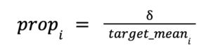
where prop_i is the proportional increase for each state or metro, δ is the coefficient of the treatment-time interaction term for the policy in question, and target_mean_i is the estimated value for the target variable for each state or metro

We computed a mean proportion for the top 3 treated states or metros:

where mean_prop is the calculated mean proportion, prop_i_1, prop_i_2, prop_i_3 are the proportion for the top 3 states or metros.

That proportional effect was added to the estimated mean funding, jobs, exits and entrepreneurial rate by multiplying the averaged proportion with the estimated value for each and added to the respective estimated value for every untreated state.

where counterfactual_i is the estimated value for the untreated state or metro if it were to receive treatment, target_mean_i is the estimated value for the untreated state or metro for the given target variable, mean_prop is the calculated mean proportion.

We compiled all the significant counterfactuals for the untreated states. To compute the counterfactual total values, mean funding and mean jobs need to be multiplied by the number of founders to obtain total funding and jobs, and entrepreneurial rate needs to be multiplied by the population per 100K to obtain total founders (see above).

These final values become our estimated increase in total funding, total jobs, total founders and mean exits if an untreated state or metro were to implement such a policy.

Join StartOut

Almost every LGBTQ+ entrepreneur has encountered unequal access to key resources needed to advance their business.